In the RNN lesson we have seen how to use a Recurrent Neural Network to perform sentiment analysis over a dataset of simple sentences written in English. Now it is time to change the language!
from tqdm.notebook import trange
import pandas as pd
import torch
import torch.nn as nn
import torch.optim as optim

seed = 314
device = "cpu"
path = "/content/drive/<path to the sentiment dataset>/Sentiment/"
The dataset we are going to use is an Italian translation of the previous dataset. The translation is a bit maccheroni-like, in order to keep the dataset simple, with a limited vocabulary size.
trset = pd.read_csv(path + "train_it.csv")
tsset = pd.read_csv(path + "test_it.csv")
tsset
| sentence | sentiment | |
|---|---|---|
| 0 | questo è felice | 1 |
| 1 | sto bene | 1 |
| 2 | questo non è felice | 0 |
| 3 | non sto bene | 0 |
| 4 | questo non è male | 1 |
| 5 | non sono triste | 1 |
| 6 | sto molto bene | 1 |
| 7 | questo va molto male | 0 |
| 8 | sono molto triste | 0 |
| 9 | questo va male non bene | 0 |
| 10 | questo va bene e è felice | 1 |
| 11 | non sto bene e non sono felice | 0 |
| 12 | non sono per niente triste | 1 |
| 13 | questo non va per niente bene | 0 |
| 14 | questo non va per niente male | 1 |
| 15 | questo va bene ora | 1 |
| 16 | questo è triste ora | 0 |
| 17 | questo va molto male ora | 0 |
| 18 | questo non andava bene prima | 1 |
| 19 | non ero felice e non andava bene prima | 0 |
Embedding
The addressed task is still binary sentiment analysis. In order to work with this slightly harder dataset, however, we will use a more powerful embedding technique.
Instead of trying to guess a good embedding for the task, we can integrate the embedding task in the model, and let the Gradient Descent learn it along with the task-related weights.
To accomplish this, we apply the same approach used in the MLP for classifying the XOR dataset, adding an initial layer of perceptrons that takes the one-hot word embeddings and map them in an embedding space.
In PyTorch, you can use nn.Embedding to perform the one-hot encoding and the
linear mapping 1. This layer takes in input the vocabulary index of a word
and return the corresponding embedding.
Let’s define again the auxiliary functions to generate the vocabulary, and the conversion of a sentence into a list of vocabulary indices.
def mapping(trset):
  sentences = " ".join(s for s in trset["sentence"])
  vocabulary = set(sentences.split(" "))
  voc_size = len(vocabulary)
  voc_idx = {w: i for i, w in enumerate(vocabulary)}
  return voc_idx, voc_size


def sentence2ids(sentence, voc_idx):
  words = sentence.split(" ")
  return torch.tensor([voc_idx[word] for word in words])

voc_idx, voc_size = mapping(trset=trset)
trcorpus = [sentence2ids(sentence, voc_idx) for sentence in trset["sentence"]]
tscorpus = [sentence2ids(sentence, voc_idx) for sentence in tsset["sentence"]]
Model
In addition to a new embedding, we introduce a new recurrent model.
One of the principal obstacle in the RNN learning, is due to a well-known problem called vanishing/exploding gradient. In simple words, when it is computed, the gradient associated to the first words of a sentence tends to:
- vanish: in such case, the model weights are updated mostly by the most recent words of a sentence that the model has received as input, failing to learn the desirable long-term dependencies that we have discussed in the previous lessons.
- explode: in this case, instead, the learning tends to become unstable and may not even converge.
The effects of vanishing/exploding gradients are similar to those related to the choice of a bad learning rate. However, while in the exploding case there exist established techniques for keeping the gradient under control, in the vanishing case, things are a bit complex and the possible mitigations usually depend on the task.
In the case of sequence learning, a new model architecture, called Long Short-Term Memory (LSTM) has been proposed by Hochreiter and Schimdhuber in the late ’90s.
The LSTM works in the same way of an RNN. It takes in input the sentence word-by-word, and propagates a hidden output $\vec{h}^{(t)}$, that can be used to generate the network outputs. In addition, the model propagates, in parallel with $\vec{h}^{(t)}$, another hidden output, called cell state and defined by $\vec{C}^{(t)}$.
The diagram of an LSTM cell is the following 2:
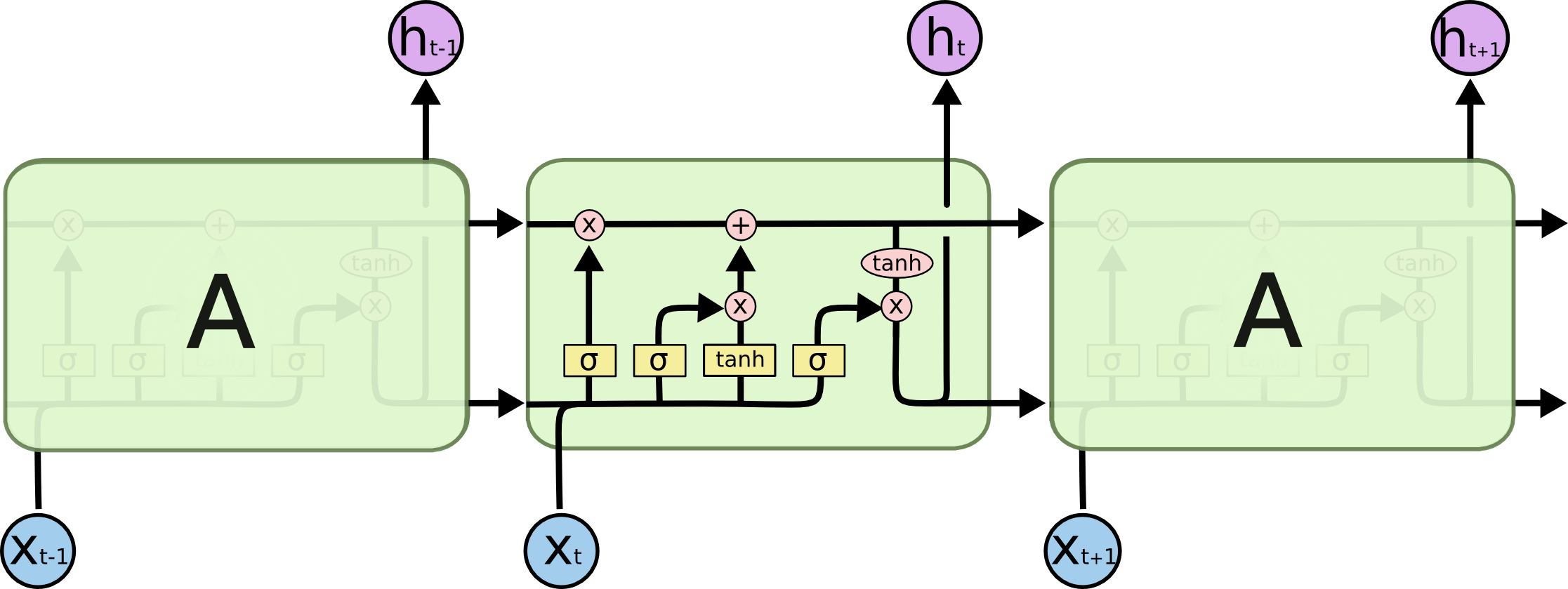
Although difficult at first sight, the structure can be decomposed in three parts, each devoted to a specific sub-task.
Forget gate layer
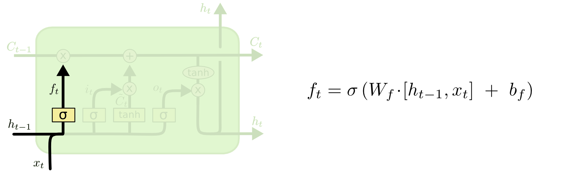
The left branch takes the hidden input $\vec{h}^{(t - 1)}$, concatenates it with the word embedding $\vec{x}^{(t)}$ (the concatenation is the vector $(h_1^{(t - 1)} \dots h_m^{(t - 1)}, x_1^{(t)}, \dots x_d^{(t + 1)}$) and applies a linear mapping + sigmoid.
- The sigmoid squashes everything in $(0, 1)$. These values will be used soon on the cell state components. Values next to $0$ cancel out (forget) the corresponding value of cell state, while keeping the other components
- $\vec{W}_f$ and its bias are the learning parameters for this step.
Update gate layer
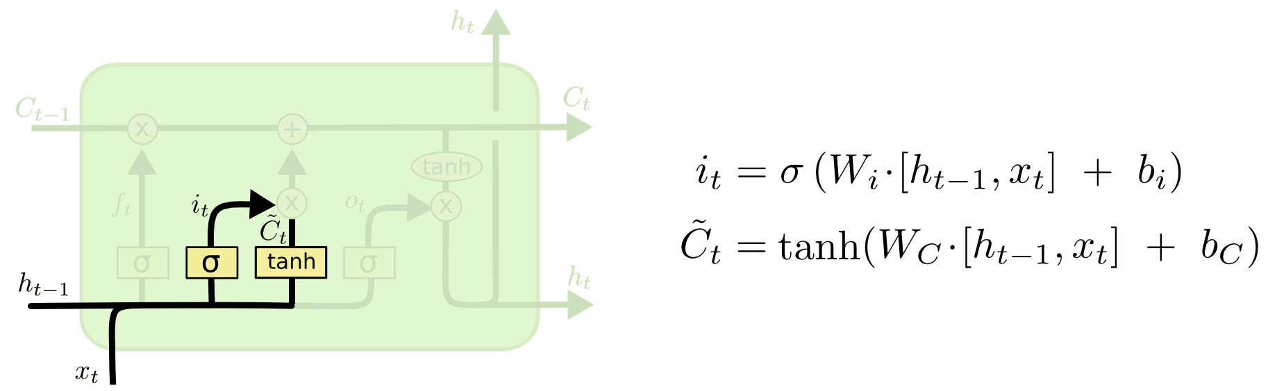
The middle branch, again, concatenates the hidden input with the word embedding and applies, two linear mappings + activation functions, separately.
- The $\tanh$ one produces updates for the each component of the cell state.
- The sigmoid one has the same effect of the forget layer and is applied to the updates in order to filter out the unwanted ones.
- $\vec{W}_i$, $\vec{W}_C$ and their biases are the learning parameters for this step.
Forget & update
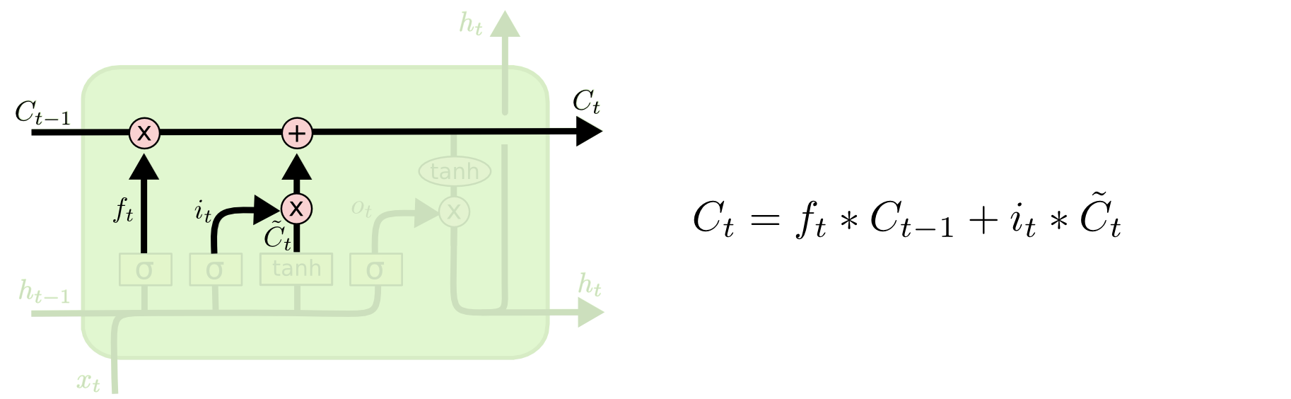
The results of the previous branches are applied to the cell state to generate the new one, $\vec{C}^{(t)}$.
Hidden and network outputs
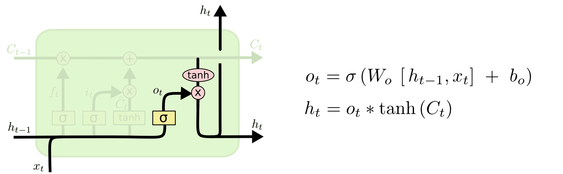
Finally the new hidden output $\vec{h}^{(t)}$ is computed using the new cell state and the previous hidden input (along with the word embedding).
- A $\tanh$ activation is applied to $\vec{C}^{(t)}$
- A linear mapping + sigmoid is applied to the concatenation of $\vec{h}^{(t - 1)}$ and $\vec{x}^{(t)}$
- the two results are multiplied element-wise to produce $\vec{h}^{(t)}$
- If needed, the network output $\vec{o}^{(t)}$ can be computed at this point with the usual linear mapping + activation function (sigmoid in the image).
This is just a standard implementation of the LSTM. In literature, you can find many variants, depending on the task.
In PyTorch, we can use the nn.LSTM layer, whose functioning resembles that of
nn.RNN (so it takes care to compute the hidden outputs only). The main
difference is that it returns the cell state, along with the hidden ouput, and
requires a dummy initial cell state $\vec{C}^{(0)}$.
class SentimentLSTM(nn.Module):
  def __init__(self, voc_size, hidden_size):
    super(SentimentLSTM, self).__init__()

    self.embedding = nn.Embedding(voc_size, hidden_size)
    self.rnn = nn.LSTM(input_size=hidden_size, hidden_size=hidden_size,
                      batch_first=True)
    self.classifier = nn.Linear(hidden_size, 1)
    self.sigmoid = nn.Sigmoid()

  def forward(self, sentence):
    sentence = self.embedding(sentence.to(torch.long))
    h0 = torch.zeros(1, 1, 64)  # initial hidden input is set to zeros values
    c0 = torch.zeros(1, 1, 64)
    _, (hn, _) = self.rnn(sentence, (h0, c0))
    prob = self.sigmoid(self.classifier(hn))
    return prob
Let’s redefine the training script used for the sentiment analysis task
def evaluate(y_true, y_pred):
  correct = (y_true == y_pred).sum()
  accuracy = 100. * correct / y_true.shape[0]
  return accuracy.item()  # returns just the value without the tensor wrapper

def train(epochs, model, trcorpus, tscorpus):
  BCE = nn.BCELoss()
  optimizer = optim.SGD(model.parameters(), lr=1e-3)

  pbar = trange(epochs, desc="E: , ACC: ")
  for epoch in pbar:
    # Training
    avg_loss = 0.
    model.train()
    for sentence, y in zip(trcorpus, trset["sentiment"]):
      sentence = sentence.to(device).to(torch.float).unsqueeze(0)
      prob = model(sentence)
      E = BCE(prob[0], torch.tensor([[y]]).to(device).to(torch.float))
      avg_loss += E.item()

      optimizer.zero_grad()
      E.backward()
      optimizer.step()

    # Evaluation
    y_true = torch.tensor(tsset["sentiment"].to_list())
    y_pred = []
    model.eval()
    for sentence in tscorpus:
      sentence = sentence.to(torch.float).unsqueeze(0)
      prob = model(sentence)
      y_pred.append(prob >= 0.5)

    y_pred = torch.tensor(y_pred)
    pbar.set_description(f"E: {avg_loss / len(trcorpus):.4f}, "
                         f"ACC: {evaluate(y_true, y_pred):.4f}")
Finally, with these two lines of code, you can run the model. With the following configuration, I was able to reach 70% accuracy, can you do better?
model = SentimentLSTM(voc_size=voc_size, hidden_size=64).to(device)
train(epochs=2000, trcorpus=trcorpus, tscorpus=tscorpus, model=model)
Note that, differently from the perceptron structure, this layer does not apply any activation function after the linear mapping. ↩︎
All images taken from this extraordinary and well-known blog post ↩︎