In this tutorial you will see how to build your first neural network, the Multilayer Perceptron (MLP), and how to use it to learn simple logical functions (AND and XOR), to correctly classify their inputs

from tqdm.notebook import tqdm
import numpy as np
import pandas as pd
import matplotlib.pyplot as plt
import seaborn as sns

import torch
import torch.nn as nn  # contains NN related stuff
import torch.optim as optim  # contains weight updaters

device = 'cpu' 
seed = 1

def set_seed(seed):
  torch.manual_seed(seed)
  torch.cuda.manual_seed(seed)
  np.random.seed(seed)

AND dataset

First of all, let’s visualize the first dataset the we are going to use: it consists of a searies of binary observations that encode the AND ($\land$) function. Every observation $\vec{x}_i$ is a 2D vector containing the inputs to the AND function, while the label $y_i$ contains the output of the function. The AND rule states that $y_i = 1$ if $x_{i1} = 1$ and $x_{i2} = 1$. For example, if $\vec{x}_i = \begin{pmatrix}0 & 1\end{pmatrix}$ then $y_i = 0 \land 1 = 0$.

The AND logic table:

$x_{i1}$	$x_{i2}$	$y_i$
0	0	0
0	1	0
1	0	0
1	1	1

You can create your dataset with the following function AND_dset that takes in input the number of observations size and a seed (seed), for experimental reproducibility. Let’s create a dataset with 100 observations (the seed has been previously set to 1)

def AND_dset(size, seed):
  set_seed(seed)
  X = torch.rand(size, 2)  # generate random matrix in [0, 1) of size x 2
  X = (X >= 0.5)  # binarize the dataset
  X = X.to(torch.float)  # convert to float
  y_true = X.prod(dim=1)  # generate the labels
  return X, y_true

X, y_true = AND_dset(100, seed)
print(X[:10], y_true[:10])

tensor([[1., 0.],
        [0., 1.],
        [0., 1.],
        [0., 1.],
        [1., 0.],
        [1., 1.],
        [1., 0.],
        [0., 0.],
        [1., 0.],
        [1., 1.]]) tensor([0., 0., 0., 0., 0., 1., 0., 0., 0., 1.])

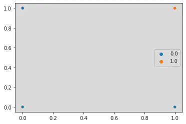
Let’s visualize the dataset with seaborn.scatterplot. Let’s use the class to compute the observations (hue parameter). Notew that the observations overlap each others, and are mapped only of four points $(0, 0)$, $(0, 1)$, $(1, 0)$, $(1, 1)$

sns.scatterplot(x=X[:, 0], y=X[:, 1], hue=y_true)

McCulloch & Pitts Neuron

A neural netwrok (NN), is one of the most used classifier nowadays.

Let’s start from the simplest model, composed by only one neuron: the M-P Neuron, invented in 1943 by McCulloch and Pitts

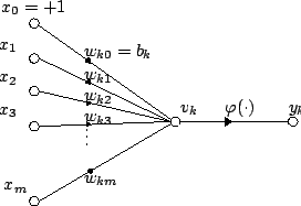
The M-P Neuron takes as input only binary observations and outputs a binary value. Its algorithm is simple:

Take an observation $\vec{x}$
Compute the aggregation function: $g(\vec{x}) = \sum_i^n x_i$
Compute the step function: $f(\vec{x}) = 1$ if $g(\vec{x}) \ge \theta$ otherwise $f(\vec{x}) = 0$.

$\theta$ is the bias, the threshold that decides if a neuron “fires” ($1$) or not ($0$). It can be learned or set by hand.

These passages form the forward step of the model

Exercise 1: M-P neuron forward step (5m)

In PyTorch, any model is a subclass of the class torch.nn.Module

When you subclass Module, you must overwrite the abstract method forward, which defines the forward step of the model, described above.

Fill in the forward method

Solution

class MPN(nn.Module):
  def __init__(self, theta):
    super(MPN, self).__init__()
    self.theta = theta

  def forward(self, x):  # x is an (n, 2) tensor
    g_x = x.sum(dim=1)
    f_x = (g_x >= self.theta).to(torch.float)
    return f_x

Let’s define also a function for computing the accuracy of the model

def evaluate(y_true, y_pred):
  correct = (y_true == y_pred).sum()
  accuracy = 100. * correct / y_true.shape[0]
  return accuracy.item()  # returns just the value without the tensor wrapper

Now, we are ready to test our model with different values of theta To call the forward step of an NN, it is sufficient to use the following code:

  model = MyNN()
  model(X)  # forward

Try to edit by hand the values of theta, until you find the one that returns 100% of accuracy.

Quiz: Can you find the minimum theta value needed to obtain 100% accuracy? Can you explain why?

theta = 2.
mpn = MPN(theta)
y_pred = mpn(X)  # calls the forward method
accuracy = evaluate(y_true, y_pred)
print(f'The accuracy with theta = {theta} is {round(accuracy, 2)}%')

The accuracy with theta = 2.0 is 100.0%

Noisy AND dataset

The AND function is rather simple to be learned. Let’s try to address a more complex problem. In real datasets, the collected observations contain noise that must be “filtered out” by the model (otherwise you get the overfitting).

Let’s generate our new dataset, which is a perturbed version of the AND dataset, previously seen

def noisy_AND_dset(size, seed, a=-2e-1, b=2e-1):
  X, y_true = AND_dset(size, seed)
  a, b = -2e-1, 2e-1  # floats in scientific notation: 2e-1 == 2 * 10 ** -1
  eps = a + (b - a) * torch.rand(X.shape)  # random noise between in [a, b)
  Xp = X + eps
  return Xp, y_true

Xp, y_true = noisy_AND_dset(100, seed)
Xp[:10], y_true[:10]

(tensor([[ 1.0484, -0.1479],
         [ 0.1708,  0.9224],
         [ 0.1205,  1.0060],
         [-0.0156,  0.9936],
         [ 1.0340,  0.0943],
         [ 1.0321,  1.0610],
         [ 0.8201,  0.1457],
         [ 0.1744,  0.1653],
         [ 1.1478, -0.1443],
         [ 0.9259,  1.1763]]),
 tensor([0., 0., 0., 0., 0., 1., 0., 0., 0., 1.]))

sns.scatterplot(x=Xp[:, 0], y=Xp[:, 1], hue=y_true)

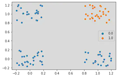
If we use the M-P neuron, the accuracy decreases

y_pred = mpn(Xp)
accuracy = evaluate(y_true, y_pred)
print(f'The accuracy with theta = {theta} is {accuracy:.2f}%')

The accuracy with theta = 2.0 is 84.00%

Perceptron

The neuron can be improved by adding learnable parameters, and a learning algorithm. First of all the forward step changes in this way:

Take an input $\vec{x}$
Compute $g(\vec{x}) = w_0 + \vec{w}^\top\vec{x} = \sum_{i=0}^n w_i x_i$, with $x_0 = 1$
Compute the thresholding function: $f(\vec{x}) = 1$ if $g(\vec{x}) \ge 0$ otherwise $f(\vec{x}) = 0$

The parameters to be learned are $\vec{w} = \begin{pmatrix}w_0 & w_1 & w_2 & \dots & w_m\end{pmatrix}^\top$. In particular, $w_0 = -\theta$, the bias that was set by hand before and now is learned together with the other parameters. In our case, $m = 2$, so we have only $3$ parameters to learn.

This model is called perceptron and has been designed by Rosenblatt in the 1958

class Perceptron(nn.Module):
  def __init__(self):
    super(Perceptron, self).__init__()
    w = torch.zeros(3)

    # special wrapper for learnable parameters. By default it requires the grad
    # but in our case we don't use it
    self.w = nn.Parameter(w, requires_grad=False)  

  def forward(self, x): # x is an (n, 2 + 1) tensor
    g_x = x @ self.w
    f_x = (g_x >= 0).to(torch.float)
    return f_x

Weight update

Now we need an algorithm to update the weights. In this case, you can use the delta-rule. The procedure is quite simple:

for $e \in {0, \dots, \mathcal{E}}$
  2. for $\vec{x}_i \in \vec{X}$
    3. $\hat{y}_i = f(\vec{x}_i)$
    4. $\vec{w}^{(e + 1)} = \vec{w}^{(e)} + \eta(y_i - \hat{y}_i)\vec{x}_i$

$f(x)$ is our perceptron, while $\vec{\eta}$ (eta) is the learning rate (lr) and it is set manually. There is not a precise rule to set it: a too small lr will slow down the convergence of the algorithm, while a too great lr can make the algorithm unable to converge.

A complete iteration over all the dataset $\vec{X}$ is called epoch (for big datasets it can take a lot of time). We can decide to repeat the algorithm for a predefined number of epochs $\mathcal{E}$ in order to improve the final performance of the network

Exercise 2: Delta-rule

Try to implement the delta rule. You have two for cycles:

The first one is on the epochs. You can use for e in range(1, epochs + 1) (remember that python starts counting from $0$).
The second is on the observations of the dataset. You can use for x, y in zip(X, y_true), that returns the single observations $\vec{x}_i$ (x) and labels $y_i$ (y).

Given a perceptron p, the delta rule consist of updating the weights of the perceptron p.w according to the rule written above

Solution

def delta_rule(X, y_true, p, epochs=1, eta=0.5, device='cpu'):
  """ X is an (n, m + 1) tensor
      y_true is an (n,) tensor
      p is the perceptron
  """
  X, y_true = X.to(device), y_true.to(device)
  for e in range(1, epochs + 1):
    for x, y in zip(X, y_true):
      y_hat = p(x)
      p.w += eta * (y - y_hat) * x  
 
  y_pred = p(X)
  print(f'ACC: {evaluate(y_true, y_pred)}')

Let’s train and evaluate the model:

def pad1(X):
  """ Pad the dataset with ones on the left"""
  return torch.cat((torch.ones(len(X), 1), X), dim=1)

p = Perceptron().to(device)
delta_rule(pad1(Xp), y_true, p, epochs=1, eta=0.05, device=device)

ACC: 100.0

# plotting the decision boundary
def plot_decision_boundary(X, y, w):
  m, q = -w[1] / w[2], -w[0] / w[2]
  x0, x1 = -2e-1, 1.2
  y0, y1 = m * x0 + q, m * x1 + q
  sns.scatterplot(x=X[:, 0], y=X[:, 1], hue=y)
  sns.lineplot(x=torch.tensor([x0, x1]), y=torch.tensor([y0, y1]), color="r")

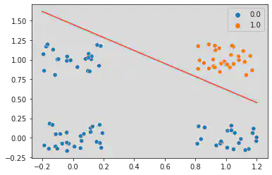
plot_decision_boundary(Xp, y_true, p.w.to('cpu'))

XOR dataset

The perceptron previously proposed allow us to solve a generic problem of binary classification, given that it is linearly separable, that is the observation of different classes must be separable by a line. If we try, for example, to learn an XOR function, that returns $1$ if, between the two inputs, only one is set to $1$, the perceptron fails

Logic table of XOR:

$x_{i1}$	$x_{i2}$	$y_i$
0	0	0
0	1	1
1	0	1
1	1	0

def XOR_dset(size, seed):
  X = torch.rand(size, 2)  # pun intended here :D
  X = (X >= 0.5).to(torch.float)
  y_true = X.sum(dim=1) % 2
  return X, y_true
  
Xor, yor_true = XOR_dset(100, seed)
Xor[:10], yor_true[:10]

(tensor([[0., 1.],
         [1., 0.],
         [0., 0.],
         [0., 0.],
         [1., 0.],
         [0., 1.],
         [1., 0.],
         [1., 1.],
         [0., 1.],
         [0., 0.]]), tensor([1., 1., 0., 0., 1., 1., 1., 0., 1., 0.]))

sns.scatterplot(x=Xor[:, 0], y=Xor[:, 1], hue=yor_true)

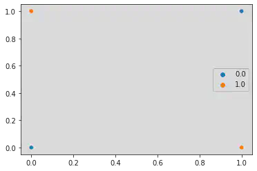
The problem is not separable with a line, therefore I cannot use the perceptron.

Multilayer Perceptron

To solve such problem we are going to modify the algorithm in two ways:

We will replace the step function with a more generic non-linear activation function
We will replace the delta-rule with the Gradient Descent (GD) algorithm

Activation function

In place of the step function, we are going to use the sigmoid function, that we have seen in the previous lessons:

$$\sigma(x) = \frac{1}{1 + e^{-x}} = \frac{e^x}{e^x + 1}$$

xs = torch.linspace(-10, 10, 1000)
y_step = (xs >= 0).to(torch.float)
y_sig = torch.sigmoid(xs)

sns.lineplot(x=xs, y=y_step)
sns.lineplot(x=xs, y=y_sig)
plt.legend(('step', 'sigmoid'))

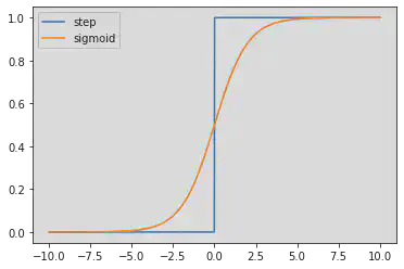
The sigmoid is a “soft” version of the step function, but it is differentiable! This is needed to use the GD algorithm

This is, however, not enough, as our perceptron is not enough flexible. Our model has only one neuron, and it is time to make it more “intelligent”, by adding more neurons

This is our new architecture:

The model is called Multilayer Perceptron (MLP) and it is composed of:

input layer: the observation $\vec{x}_i$.
hidden layer: $\vec{h}_i$ composed of two perceptrons. Each of them takes the same input $\vec{x}_i$ and returns a value.
output layer: it behaves like the previously seen perceptron, but instead of using the $\vec{x}_i$, it processes $\vec{h}_i$.
Each neuron applies the aggregation and the sigmoid function to their respective inputs.

An MLP can have more neurons and more layers. For our task, it is sufficient that shown in figure

In PyTorch, to build the hidden/output layer we can use: torch.nn.Linear and torch.sigmoid, as follows:

class MLP(nn.Module):
  def __init__(self):
    super(MLP, self).__init__()
    self.hidden_layer = nn.Linear(2, 2)  # x --> h 
    self.output_layer = nn.Linear(2, 1)  # h --> y_hat
    self.sigmoid = nn.Sigmoid()

  def forward(self, x):
    h = self.sigmoid(self.hidden_layer(x))
    y_hat = self.sigmoid(self.output_layer(h))
    return y_hat

Now let’s illustrate the Gradient Descent algorithm. It is similar to the delta rule:

for $e \in {0, \dots, \mathcal{E}}$
  2. $\hat{\vec{y}} = f(\vec{X})$
    3. $E(f) = MSE(\hat{\vec{y}}, \vec{y})$
    4. $\vec{w}^{(e + 1)} = \vec{w}^{(e)} - \eta \nabla_\vec{w}{E(f)}$

$E(f)$ is the Mean Squared Error (MSE) loss. The greater its value, the worse our predictions. Our objective consists of minimizing it bringing as close as possible to $0$.
$\nabla_\vec{w}{E(f)}$ is the gradient, that is a vector containing the derivatives of $E(f)$ for all $w_j$. We do not compute it manually, PyTorch takes care of it

Exercise: MLP Training (10m)

Try to implement the training of the algorithm: 0. Create MSE = torch.nn.MSELoss() to compute the MSE, and GD = torch.optim.SGD(p.parameters(), lr=eta) to update the weights

For cycle on the epochs
Forward step of the MLP, where we input all the dataset X at once
Compute the MSE, by calling E = MSE(y_hat, y_true)
Compute the gradient by calling E.backward() and then update the weights with GD.step(). After this, call a magic command GD.zero_grad().

def train(X, y_true, p, epochs=1, eta=0.5, device='cpu'):
  X, y_true = X.to(device), y_true.to(device)
  # 0.
  ...
  ...
 
  # display a progress bar during the model training
  prog_bar = tqdm(range(epochs), total=epochs, desc=f'E: , ACC: ')
  for e in prog_bar:  # 1.
    p.train()  # switch the model to training mode
    # 2.
    ...

    # 3.
    ...
    # 4.
    ...

    ...
    ...

    p.eval()  # switch the model to evaluation mode

    # Evaluation
    y_pred = p(X).round().flatten()  # predict based on the sigmoid values
    prog_bar.set_description(f'E: {E.item():.4f}, '
                             f'ACC: {evaluate(y_true, y_pred)}%')

Solution

def train(X, y_true, p, epochs=1, eta=0.5, device='cpu'):
  X, y_true = X.to(device), y_true.to(device)
  # 0.
  MSE = nn.MSELoss()
  GD = optim.SGD(p.parameters(), lr=eta)
 
  # display a progress bar during the model training
  prog_bar = tqdm(range(epochs), total=epochs, desc=f'E: , ACC: ')
  for e in prog_bar:  # 1. for cycle on epochs
    p.train()  # switch the model to training mode
    y_hat = p(X).flatten()

    E = MSE(y_hat, y_true)  # compute the (expected) loss
    E.backward()  # backpropagation: compute the gradient

    GD.step()  # update the weights
    GD.zero_grad()  # magic command remember to call it!

    p.eval()  # switch the model to evaluation mode

    # Evaluation
    y_pred = p(X).round().flatten()  # predict based on the sigmoid values
    prog_bar.set_description(f'E: {E.item():.4f}, '
                             f'ACC: {evaluate(y_true, y_pred)}%')

With the following code, you can run the Gradient Descent. Providing enough epochs, you should be able to reach 100% accuracy ✌️

mlp = MLP().to(device)
train(Xor, yor_true, mlp, epochs=6000, eta=1.5, device=device)

Multilayer Perceptrons

AND dataset

McCulloch & Pitts Neuron

Exercise 1: M-P neuron forward step (5m)

Noisy AND dataset

Perceptron

Weight update

Exercise 2: Delta-rule

XOR dataset

Multilayer Perceptron

Activation function

Exercise: MLP Training (10m)