K-Nearest Neighbors (KNN) is a classification model designed in the 1951, and based on a very simple classification rule. In this lesson, we will see how to use it to perform text genre classification.

Dataset

First of all let’s have a look at the dataset, called 20newsgroups. It is a standard text dataset used to perform simple ML tasks. scikit-learn provides it through the fetch_20newsgroups function, which requires a path where to store the dataset.

from sklearn.datasets import fetch_20newsgroups
path = "drive/MyDrive/<path where to store my datasets>"
bunch = fetch_20newsgroups(data_home=path, subset="train")
bunch_test = fetch_20newsgroups(data_home=path, subset="test")

The dataset behaves like a Python dictionary and contains three important fields:

data: the actual data, consisting of around 18000 small newsgroups posts regarding different topics.
target: the ground truth for each post, regarding its topic. There are 20 topics in total.
target_names: the name of each topic.

print(bunch["target_names"])

['alt.atheism', 'comp.graphics', 'comp.os.ms-windows.misc', 'comp.sys.ibm.pc.hardware', 'comp.sys.mac.hardware', 'comp.windows.x', 'misc.forsale', 'rec.autos', 'rec.motorcycles', 'rec.sport.baseball', 'rec.sport.hockey', 'sci.crypt', 'sci.electronics', 'sci.med', 'sci.space', 'soc.religion.christian', 'talk.politics.guns', 'talk.politics.mideast', 'talk.politics.misc', 'talk.religion.misc']

Text Preprocessing

When working with documents two preprocessing steps must be performed:

Tokenization: the splitting of the document string into small chunks. Each token should, in principle, represent the same “unit” of text data (word, sentence, etc.). In our case, we will split each document into lowercase words, without any other specific transformation.
Embedding: the conversion of the document tokens into a vector of values, in order to be able to feed the input to an ML model. This conversion usually takes into account relationships among the tokens.

Embedding

For the embedding we are going to use the Term Frequency Inverse Document Frequency (TFIDF) embedding. Given a corpus of documents $D = {d_1, \dots, d_n}$ and a word $w_j$, the tfidf value of $w_j$ with respect to a document $d_i$ is

$$tfidf(w_j, d_i) = tf(w_j, d_i)idf(w_j, D)$$

$tf$ stands for term frequency, it is the relative frequency (percentage) of occurrences of the term $w_j$ in document $d_i$, and it is computed as the absolute frequency $n_{ij}$ (number of occurrences) of $w_j$ in $d_i$ divided by the total number of words in $d_i$:
$$tf(w_j, d_i) = \frac{n_{ij}}{|d_i|}$$
The rationale is that a word that appears more often in a document, must be more indicative of the document topic. For example, a document about cars should contain more occurrences of the word ‘car’, ‘tire’, ‘road’, etc. with respect to a document about politics.
$idf$ stands for inverse document frequency and it is meant to adjust the term frequency in order to not take into account very common words, such as articles (e.g. ‘the’, ‘a/an’) auxiliary verbs (e.g. ‘be’, ‘have’), and so on. We first start by computing the relative frequency of how many documents in the corpus contain the word $w_j$, that is $|\{d \in D \mid w_j \in d\}| / |D|$. The numerator reads the number of documents that contain word $j$, while the denominator is the number of documents composing the corpus $D$. idf computes the logarithm of the inverse ratio mentioned above:
$$idf(w_j, D) = \ln\left(\frac{|D|}{|\{d \in D \mid w_j \in d\}|}\right)$$
Such quantity is important in the context of information theory and measures the “surprise” that an event with relative frequency $p$ bears. Intuitively, an event that happens rarely (e.g. an earthquake) bears much more surprise than a common event (e.g. the sunset in the evening). Thus with this quantity we can downweigh very common words that occurs in the majority of documents, while retaining the rare ones. These quantities, multiplied together, give rise to the tfidf index: the frequency of a term multiplied by the surprise of finding it in a document.

In scikit-learn, we can compute the tfidf index using TfidfVectorizer, which provides a matrix of size $n \times v$ where $n$ is the number of documents (observation) and $v$ is the vocabulary size (number of distinct words in the corpus). We can also specify a max_features parameter to provide an upper bound on the number of features $v$ ordered by term frequency across the corpus. You run the transformation calling the fit_transform method, then you can apply the transformation on new (test) data with the transform method.

from sklearn.feature_extraction.text import TfidfVectorizer
tfidf = TfidfVectorizer(max_features=10000)

# Training set
X = tfidf.fit_transform(bunch["data"])
y = bunch["target"]

# Test set
X_test = tfidf.transform(bunch_test["data"])
y_test = bunch_test["target"]

Model

The classifier we are going to use is called K-Nearest Neighbors (KNN). It is a non-parametric model, meaning that it has not learnable parameters. The classification rule is very simple but effective: upon given a new observation, check the class of its $k$ nearest observations in the training set (neighbors). The majority class of the neighbors determines the assigned class. This is the simplest form of KNN, but there are many variants we will not discuss here.

scikit-learn provides the class KNeighborsClassifier which requires to set two fundamental parameters: the number of neighbors $k$ (n_neighbors), and the distance function used to determine the neighbors (metric)

from sklearn.neighbors import KNeighborsClassifier
knn = KNeighborsClassifier(n_neighbors=5, metric="cosine")
knn.fit(X_train, y_train)
knn.score(X_test, y_test)

0.6383430695698353

Validation

After having performed the embedding, we split the dataset into training and test set with train_test_split

n_neighbors and metrics are not learned, though they determine the classification performance of the algorithm. Such parameters are called hyperparameters and every ML algorithm requires to set some of them. In the case of the regression, for example, the degree of the non-linear models is an hyperparameter. The setting of hyperparameters is crucial and determines the overfitting, or its opposite, unwanted phenomenon, the underfitting, that happens when a model is too rigid and is not able to learn at all the underlying pattern that models the data.

In the case of KNN, for example, if we set $k = 1$, the algorithm classifies an observation based on its nearest neighbor class, becoming too sensible and more prone to overfit. On the other way around, if $k$ is set to the size of the training set, the algorithm classifies every observation based on the majority class in the dataset, thus underfitting the data.

How can we choose the correct value of $k$? We could be tempted to try different configurations of $k$ and evaluate the performance on the test set. However, we could incur in overfitting the test set by involuntarily choosing a favorable hyperparameter configuration, without effectively knowning the performance of the method against unseen data.

To solve this problem, we use instead a subset of the training data, called validation set with the only purpose to validate (test) multiple configuration of hyperparameters. The best one is then tested against the test set to get the performance of the model on unseen data.

This procedure is called Hyperparameter optimization/tuning (HPO/HPT), and it can be costly in terms of computational time. Indeed, for each configuration we need to train a model from scratch. We can perform a grid search by running an HPO over a range of configurations ($k \in [1, \dots, n]$), or we can just randomly sample a set of configurations, thus performing a random search. While the former approach is exhaustive and more accurate, the latter one has shown to provide very good performance, and is usually adopted in real-world training cases.

In scikit-learn, we use GridSearchCV (or RandomSearchCV), as follows:

from sklearn.model_selection import train_test_split, GridSearchCV
param_grid = {
  "n_neighbors": range(1, 50),
  "metric": ("euclidean", "cosine")
}
ids = range(len(y))
ids_train, ids_val = train_test_split(ids, test_size=0.1, random_state=42)
# This command takes a lot of time, you can set verbose=2 to check its progress
cv = GridSearchCV(knn, param_grid, cv=[(ids_train, ids_val)])
cv.fit(X, y)
cv.score(X_test, y_test)

0.6395379713223579

Visualization

The data we have used consists of a matrix of size $n \times v$, so its visualization, as it is, is hard and cumbersome. Luckily, we can use some visualization methods, that project the $v$-dimensional observations into $2$-d approximation, preserving, as much as possible, their geometry in the $v$-dimensional space. The algorithm of choice in this case is T-SNE.

The theoretical details are not in the scope of this lesson, so we will skip them. In scikit-learn, you can use this visualization method with TSNE:

from sklearn.manifold import TSNE
tsne = TSNE(n_components=2, metric="cosine")
f = tsne.fit_transform(X)

The fit_transform method produces the equivalent $2$-d approximations of the $v$-dimensional feature embeddings. After this, it is just a matter of plotting the coordinates and their classes.

import seaborn as sns
# sns.set(rc={"figure.figsize": (22, 13), "axis": "off"})
sns.set_theme(style="white")
sns.relplot(x=f[:, 0], y=f[:, 1], hue=y, palette='tab20', kind='scatter', height=10, aspect=1)

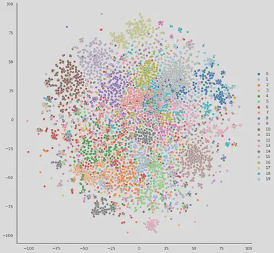
As you can see, the tfidf observations form quite recognizable groups, aiding ML algorithms in the classification.